## Warning: NAs introduced by coercion

## Warning: NAs introduced by coercion
Introduction
When the Golden State Warriors won their third championship in four years, discussions among NBA fans and commentators alike tried to locate the crux of their unprecedented success. In some spheres, the team was referred to as “tech’s team”, and writers pointed to the Bay Area’s economic success as a reason for the team’s success, and for resentment to build in other parts of the country. In fact, the Bay Area ranks 19th in the world for GDP, when compared to other countries. Fans and opponents alike wondered if there was a correlation between the high level of economic growth and the high level of basketball performance in the Bay Area? In our work, we seek to investigate the relationship between a city’s socioeconomic performance and the performance of its NBA team.
Does a metropolitan area’s socioeconomic prosperity correlate with the performance of its NBA team?

Motivation
Our study is motivated by a deep debate already existing in the sports world: Are professional teams actually good for the cities they inhabit? On the one hand, some argue that the presence of teams can draw tourism, create thriving retail businesses and boost local morale. On the other hand, some argue the presence of teams can drain taxpayer dollars that could have been allocated elsewhere. We hope that people, even those with little understanding of professional basketball, will gain a better sense of the complex interactions and relationships between cities and teams.
Data
Our data combines two very different sources to create a novel interpretation of both NBA team success and socioeconomic prosperity.
Sourcing
From a sourcing perspective, we brought in data from a variety of locations. On one side, we collected NBA data through an online repository of statistics. This helped us organize the various teams each season, how well they performed, and what arenas, and therefore cities, they play in. On the other hand, we collected socioeconomic data from a variety of different sources. We used a wide array of types of data, in order to obtain a robust view of an area’s economic success. For example, we investigated unemployment rates through the Bureau of Labor Statistics. In addition, we explored personal income levels through the Bureau of Economic Analysis. We also added drug overdose rates (per 100,000 citizens) by county from the Center for Disease Control and Prevention. We included poverty rate estimates by county from the Census Bureau. Finally, we included the percentage of citizens on food stamps from the Census Bureau to round out our analysis.
Wrangling
From a wrangling perspective, we cleaned our data extensively to allow it to be easily combined between the two distinct types. On one side, we used iterative loops to integrate basketball data from each season, as seen below.
#create vector for urls and initialize variables for loops
nba_urls <- vector(mode="list", length = 20)
j <- 1
i <- 1
k <- 1
l <- 1

#run loop to write urls for NBA stats following same patterns
for (j in j:11) {
  nba_urls[j] <- paste0("https://www.basketball-reference.com/leagues/NBA_200", j-1, ".html")
}
for (j in j:20) {
  nba_urls[j] <- paste0("https://www.basketball-reference.com/leagues/NBA_20", j-1, ".html")
}

#loop through urls and add data to the end of a common data table
nba_stats <- data.frame()
for (i in i:20) {
  url <- toString(nba_urls[i])
  url_html <- read_html(url)
  nba_tables <- html_nodes(url_html, "table")
  east_table <- html_table(nba_tables[[1]]) %>%
    clean_names() %>%
    mutate(conference="east") %>%
    rename(team=eastern_conference) %>%
    filter(!team %in% c("Atlantic Division", "Central Division", "Southeast Division"))
  west_table <- html_table(nba_tables[[2]]) %>%
    clean_names() %>%
    mutate(conference="west") %>%
    rename(team=western_conference) %>%
    filter(!team %in% c("Midwest Division", "Pacific Division", "Northwest Division", "Southwest Division"))
  stats <- rbind(east_table, west_table) %>%
    select(team, conference, w, l, w_l_percent, ps_g, srs) %>%
    mutate(team=substr(team, 1, nchar(team)-4)) %>%
    separate(team, c("team1", "team2", "team3")) %>%
    replace_na(list(team3="")) %>%
    unite("team", c("team1", "team2", "team3"), sep=" ") %>%
    mutate(year=i-1)
  nba_stats <- rbind(nba_stats, stats)
}
On the other side, we brought in disparate data sources containing
socioeconomic data that was much easier to clean. We could either apply
the above looping process to urls that corresponded to relevant years,
or we could import csv files readily available online.
One of the more difficult wrangling tasks was integrating these two data
sources together. FIPS (Federal Information Processing System) codes
assign a five digit value to each county in the US. The first two digits
correspond to the state, while the next three digits correspond to the
county. This allows the US government to organize data, especially
census statistics, in an easily-accessible manner. Luckily, this FIPS
code was already present in our socioeconomic data. However, we had to
write certain functions to translate the coordinates we found for each
NBA arena into a county name that could then be translated into the
universal FIPS code.
# create function for transposing coords to FIPs
# adapted from https://stackoverflow.com/questions/23068780/latitude-longitude-coordinates-to-county-in-r
latlong2county <- function(pointsDF) {
  # Prepare SpatialPolygons object with one SpatialPolygon
  # per county (plus DC, minus HI & AK)
  counties <- map('county', fill=TRUE, col="transparent", plot=FALSE)
  IDs <- sapply(strsplit(counties$names, ":"), function(x) x[1])
  counties_sp <- map2SpatialPolygons(counties, IDs=IDs,
                                   proj4string=CRS("+proj=longlat +datum=WGS84"))

  # Convert pointsDF to a SpatialPoints object
  pointsSP <- SpatialPoints(pointsDF,
                            proj4string=CRS("+proj=longlat +datum=WGS84"))

  # Use 'over' to get _indices_ of the Polygons object containing each point
  indices <- over(pointsSP, counties_sp)

  # Return the county names of the Polygons object containing each point
  countyNames <- sapply(counties_sp@polygons, function(x) x@ID)
  countyNames[indices]
}
Once we had ensured that FIPS codes were consistent across datasets, we then joined them by code and by year, so that for every team and for every year we had a variety of measures of success on and off the court. The first few observations can be seen below:
| Team | Conference | Year | Wins | Losses | WinLossPercentage | PointsPerGame | SimpleRatingSchedule | Rank | Arena | Attendance | AttendancePerHomeGame | County | FipsCode | UnemploymentRate | Income | OdRate | PovertyRate | Population | Percentage |
|---|---|---|---|---|---|---|---|---|---|---|---|---|---|---|---|---|---|---|---|
| Miami Heat | east | 2000 | 52 | 30 | 0.634 | 94.4 | 2.75 | 8 | AmericanAirlines Arena | NA | NA | florida,miami-dade | 12086 | 4.3 | 26614 | NA | NA | 2259508 | 0.1131052 |
| New York Knicks | east | 2000 | 50 | 32 | 0.610 | 92.1 | 1.30 | 11 | Madison Square Garden (IV) | NA | NA | new york,new york | 36061 | 5.0 | 88609 | NA | NA | 1540547 | 0.0960289 |
| Philadelphia 76ers | east | 2000 | 49 | 33 | 0.598 | 94.8 | 1.02 | 14 | First Union Center | NA | NA | pennsylvania,philadelphia | 42101 | 5.5 | 25372 | NA | NA | 1514563 | 0.1696146 |
| Orlando Magic | east | 2000 | 41 | 41 | 0.500 | 100.1 | 0.43 | 15 | TD Waterhouse Centre | NA | NA | florida,orange | 12095 | 3.1 | 27699 | NA | NA | 903019 | 0.0411951 |
| Boston Celtics | east | 2000 | 35 | 47 | 0.427 | 99.3 | -1.00 | 20 | FleetCenter | NA | NA | massachusetts,middlesex | 25017 | 2.2 | 47199 | NA | NA | 1467248 | 0.0140515 |
Findings
To depict our findings, we have built an interactive Shiny app that allows the user to explore teams and metrics of interest.
For some static results, however, there are a few examples we can walk through. First, to cirlce back our motivation as discussed earlier, let’s look at the Golden State Warriors and the Bay Area. Below is a plot illustrating the fairly rapid increase of average wealth in San Fransisco over the last few years - may this may translate into greater success for the Warriors?
## Warning: Removed 1 rows containing missing values (geom_path).
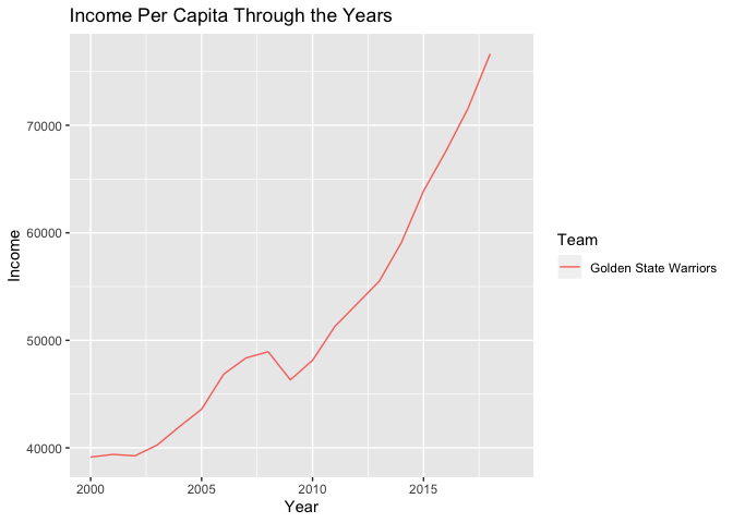
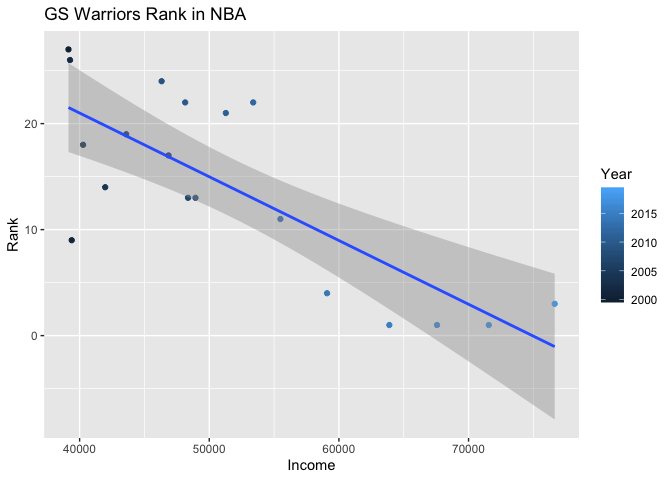
Based on a first glance at the graph below, it looks like the answer to that question is yes. As income in the county has increased over time (the light blue points signifying more recent years are clustered at high income levels), the Warriors have transformed from a team ranked in the bottom half of the league, to a consistent top 5 team. The negative relationship between income and NBA rank is rather strong in this case, making it easy to see why pundits are quick to see a link between these variables.
## Warning: Removed 1 rows containing non-finite values (stat_smooth).

## Warning: Removed 1 rows containing missing values (geom_point).
Observing these factors for the league as a whole, however, tells a different story. When every team is included, we instead see a slightly positive relationship between income and rank, suggesting that individuals counties that are better off may be cheering for teams at more towards the bottom of the pile. That being said, much of this positive trend can be attributed to a few high-leverage points, which have very high income levels and poor NBA rankings (populating the top right of the graph). Can you guess which team makes up most of this group of points?
## Warning: Removed 29 rows containing non-finite values (stat_smooth).

## Warning: Removed 29 rows containing missing values (geom_point).
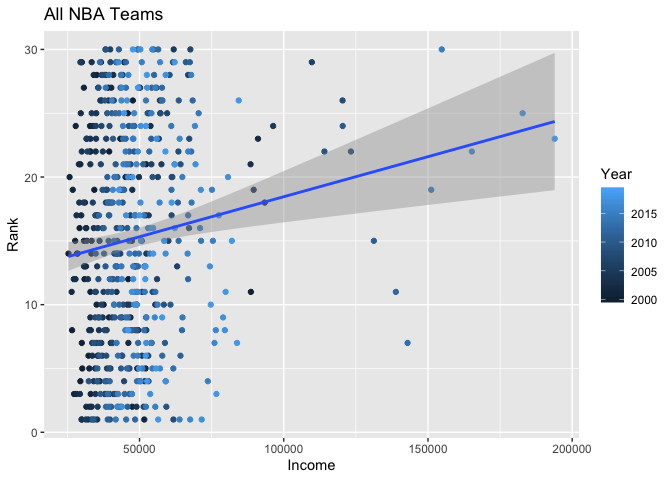
Those would be the New York Knicks, which Knicks fans probably didn’t need to be told again. Despite the high average income of Midtown New York, the Knicks haven’t been able to show much success in our time frame.

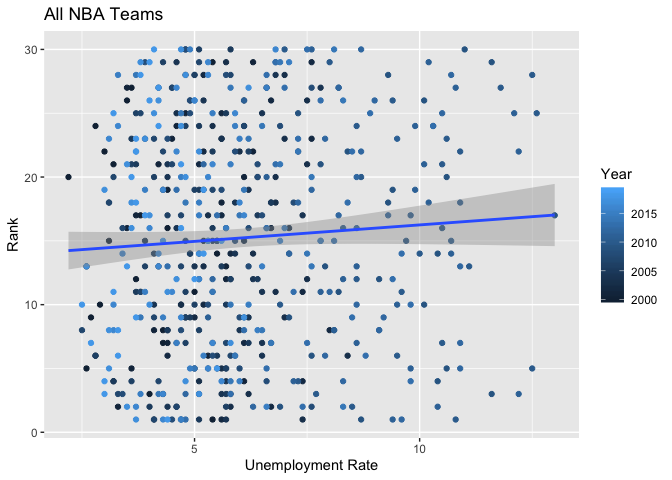
Moving on, one feature that our time frame does capture is the Economic Recession of 2008. And in our dataset, this event is likely most directly captured by Unemployment Rates, which spike in 2008 and generally stay high for a few years after.
## Warning: Removed 14 rows containing missing values (geom_path).
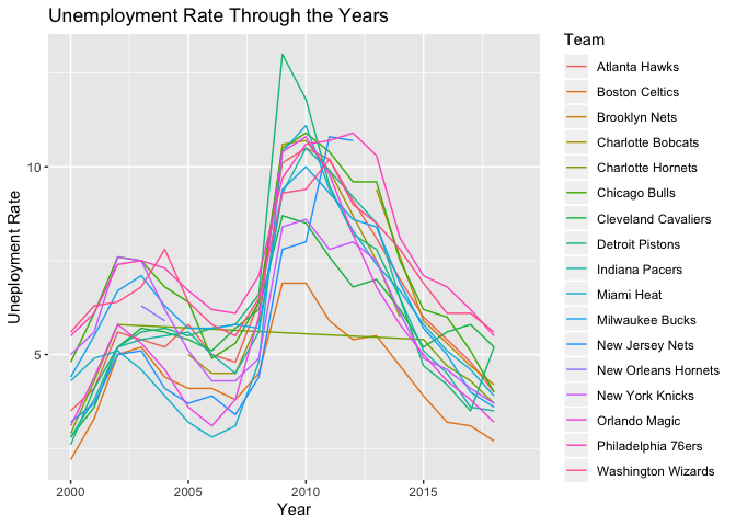
Shown above, the city of Detroit (home of the Pistons) was likely hit the hardest by the financial crisis, with unemployment maxing out at over 15 percent soon after the crash. Perhaps we may suspect the opposite effect compared to that of the Warriors, and that Detroit’s economic struggles may correspond with decreased performance in the NBA.
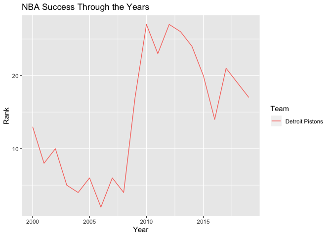
Turns out that we see exactly that. One of the top teams in the league in the years immediately prior to 2008, the Pistons quickly fell to one of the worst in the next few years. Now, can we say definitively that the decline of the Pistons was a result of financial troubles and a shortage of jobs in Detroit? Not exactly. We can’t rule out a multitude of other factors, such as possible poor trades, contracts expiring, or changes in strategy that might have just happened to occur at the same time. And again, once we add in the entire league to get a larger picture of this relationship, the evidence is less convincing. There is still a slight positive correlation between having a high unemployment rate and a high NBA rank, but the points appear to be spread quite randomly across the graph, and the confidence interval is wide enough that there could be no effect at all.
## Warning: Removed 30 rows containing non-finite values (stat_smooth).

## Warning: Removed 30 rows containing missing values (geom_point).
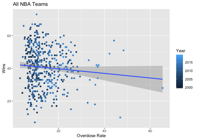
With certain teams included, one can one of our strongest correlations by plotting overdose rate and wins. And surprisingly, in those cases the correlation is positive, which makes little sense intuitively. By plotting all teams, once again, this correlation becomes very weak and actually switches to a slightly negative relationship, which is more in line with expectations.
## Warning: Removed 140 rows containing non-finite values (stat_smooth).

## Warning: Removed 140 rows containing missing values (geom_point).
Conclusion
In the end, we are not able to settle the debate conclusively on the relationship between socioeconomic data and NBA team success. While there are plenty of examples of correlations between individual teams and the conditions of their home counties, these correlations break down when more data points are added. This might explain why sports writers are quick to see relationships, as they likely draw these conclusions off of somewhat anectodal evidence for just a team or two. With a wider lense, however, we think that there are more factors that have strong impacts on NBA success that are not confined to the county level. Skill, hardwork, and strategy are likely still more important predictor variables for NBA teams to consider. Even for the variables in our dataset where we find a clearer relationship, wins and overdose rate, we are lacking data in this area and cannot suggest a reason why we might find this correlation.
Limitations
There are a number of limitations to our analysis. First, we run into the issue that some teams play in the same arena, but may achieve greatly different results. The LA Lakers and LA Clippers, for example, both play in the Staples Center, but in our time frame the Lakers have been much more successful than the Clippers. To some extent, examples like this prove that socioeconomic factors have limited impacts, so drawing conclusions in this project would be difficult.
Additionally, our data comes with a few complications, such as how different teams have different geological scopes. Specifically, sometimes the stadiums that teams play in are further from the fans that support them. Or, in some cases, within metro areas that are associated with teams there are wide gaps in socioeconomic prosperity, which our data does not pick up on. Lastly, our data is limited to 2000-2018, and we could only use socioeconomic variables that are measured on a year to year basis.
Future Research
This research could be extended in a few ways. The first one that comes to mind is to conduct similar analyses with different sports leagues, like the NFL or MLB. In this way, we would have more data points and could compare across leagues within a city to see if teams that share a fan base have similar outcomes. Additionally, we could make our model more robust and look for more interesting and significant relationships if we have more metrics of both NBA success and socioeconomic prosperity.
Bibliography
https://www.inc.com/jeff-bercovici/warriors-cavaliers-silicon-valley.html https://markets.businessinsider.com/news/stocks/california-economy-16-mind-blowing-facts-2019-4-1028142608 https://www.curbed.com/2018/1/30/16948360/stadium-public-funding-sacramento-kings https://si.wsj.net/public/resources/images/S1-AM668_NBA060_OR_20180609023422.jpg https://www.theatlantic.com/technology/archive/2018/11/sports-stadiums-can-be-bad-cities/576334/ https://www.basketball-reference.com/leagues/NBA_2019.html https://www.bls.gov/lau/#cntyaa https://www.bea.gov/data/income-saving/personal-income-county-metro-and-other-areas https://data.cdc.gov/NCHS/NCHS-Drug-Poisoning-Mortality-by-County-United-Sta/rpvx-m2md https://www.census.gov/data-tools/demo/saipe/#/?map_geoSelector=aa_c https://www.census.gov/programs-surveys/sahie/technical-documentation/model-input-data/snap.html http://images.nymag.com/news/sports/knicks080414_1_560.jpg