Introductory Information
When it comes to sports, there is always an argument about who is the best. The best player, the best team, the best conference, the best geographical area: these are some examples of debates regarding college football. We have explored how the strength of college football programs by state has changed over time. While college football began in the Northeast, the majority of successful Division 1 programs are now located in the South. We had not seen a visual or graphical representation of how or when this transition took place, so we constructed a time-based choropleth displaying the spatial movement of college football from its infancy in 1869 to the present day. Using a Shiny App, we were able to look at various ways to determine the strength of college football in each state. The three metrics we focused on were total wins by state, best team by state (using Sports Reference SRS rating), and average wins by state. We believe this visualization would be interesting to college football fans across the country.
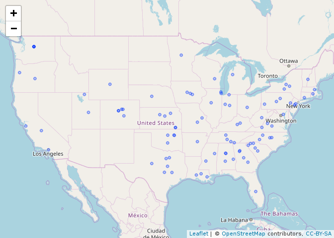
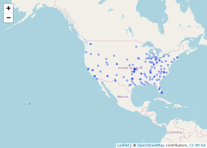
Comparing Location of Division I College Football Programs in 1920 vs 2019
The maps below show the location of Division I college football teams in 1920 and 2019. From this, we can see the evolution of schools over time. In 1920, there were very few teams out West. By 2019, we see many more teams out West (even Hawaii) and an increased number of teams throughout the country. This gives an inital look into the evolution of college football, and we investigate these changes further in our Shiny app.
#Map to show location of 1920 Division I CFB teams
teams1920 <- leaflet() %>%
  addTiles() %>%
  addCircles(lng=data1920$lon, lat=data1920$lat, radius= (data1920$Overall_W) * 500)
teams1920

# Map to show location of 2019 Division I CFB teams
teams2019 <- leaflet() %>%
  addTiles() %>%
  addCircles(lng=data2019$lon, lat=data2019$lat, radius= (data2019$Overall_W) * 500)
teams2019

Data
The data that we used comes from two primary sources. Data on the success of college programs comes from Sports Reference. The tables are organized by year (example URL: https://www.sports-reference.com/cfb/years/1869-ratings.html), providing each college with a unique ranking for their performance in a given year. We scraped this data from Sports Reference replacing “1869” in the URL with years from 1869 to 2019. We also used data from Wikipedia mapping each Division 1 program their respective state (https://en.wikipedia.org/wiki/List_of_NCAA_Division_I_FBS_football_programs).
Below is an example of the code we used to geocode and reverse geocode to get the data in the format we needed.
#Get longitude and latitude for each school
  Schoolloc<- geocode(unique(Football$School)) %>%
    mutate(School = unique(Football$School))

#Reverse geocode to get location of each school from longtitude/latitude pair
#Using help from StackOverflow to get loop, citation at bottom of blog post
result <- do.call(rbind,
                  lapply(1:nrow(Schoolloc),
                         function(i)revgeocode(as.numeric(Schoolloc[i,1:2]))))
data <- cbind(Schoolloc,result)

#Found on Stackoverflow to get state, citation at bottom of blog post
substrRight <- function(x,n){
  substr(x, nchar(x)-n+1, nchar(x))
}
Shiny App
Here is a link to our Shiny App. This allows an interactive way for the user to look at our findings.
https://tmarshall21.shinyapps.io/Shiny-app/
Findings
From our analysis, we have concluded that while the Northeast was the birthplace of college football, it is no longer the geographical center. Since the inaugural games between Princeton and Rutgers in 1869, the strength of college football has shifted out of the Northeast. We now see the best college programs located mainly in the South, but there is also a group of quality programs in the Great Lakes region and in California. Depending on the metric that is being used to evaluate teams, we get slightly different results.
For the percent of wins by state, we see that Texas and California have done very well in recent years along with a portion of the Southeast (Florida, Georgia, Alabama, etc.). The Northeast does not perform well based on this metric as we see a lot of blue in those states (indicating lower performance) and even some states that no longer have a single Division I team.This makes sense given that Texas and California are larger states and have more Division I programs than other states. There is obviously variation from year to year, but it seems that there has been a shift towards the South as the geographical center of college football.
Using highest SRS rating by state, we see similar results, but also some variation. States in the South tend to have some of the best teams (red in the Shiny app), but there are some other states that typically do very well based on this metric. Ohio is one example of this because of Ohio State which has been one of the best college football programs in the country for a while now. Other states in the Great Lakes Region such as Michigan and Wisconsin tend to perform better using this metric than the other two which is again an example of having one very strong program, but not many others in the state.
For average wins by state, we are accounting for the number of schools by state. This prevents larger states with more schools like California and Texas from performing better just because they have more teams. In this case, we again see the Northeast to be one of the worst areas in the country for college football. The South tends to be the best performing area again based on this metric, but we do see some outliers. Nebraska typically performs better based on this metric compared to others which is likely because Nebraska University is the only Division I football program in the state, so the average wins for the state of Nebraska is the number of wins for Nebraska University.
Overall, it is tough to come to a clear consensus about the geographical center of college football based on these metrics because there is variation based on the metric chosen and also year to year variation. However, we are able to conclude that the Northeast is no longer the geographical center like it was back in 1869. Now, it seems that the South is the location where the best college football programs exist. The South performed well in all three metrics we investigated demonstrated that they have a good portion of teams, some of the best teams in the country, and a good portion of successful teams in each state.
Limitations
Although we were able to make some conclusions about how college football has changed over the years, this does not necessarily translate to other sports. We would likely see different results if we were to look at college basketball, and this would be something we would be interested in looking at. This would allow us to compare across sports and determine if there is an area in the US where college sports are the strongest.
While we were able to compare states with each other, we would also be interested in comparing conferences to see how the best conferences have changed over time. This was beyond the scope of our project, but would be an intriguing extension to look at. In addition, our study could potentially be improved by finding other metrics to evaluate college football teams. We used total wins by state, best team (using SRS rating) by state, and average wins by state, but there are other ways to compare programs across state that could be interesting to investigate. For example, finding the average SRS rating of the best three teams in a state could be another way to compare across states. Potentially using other metrics to rate teams would be another possible way to extend our work.
Also, we would like to see further research on how trends in college football are connected to related trends. For example, did the rise of Mississippi’s college football programs (Ole Miss, Mississippi State, etc.) result from or result in increased high school football participation rates in the state? Does the proximity to an NFL team impact the strength of a college program? These are a couple other questions that would be interesting to explore use our analysis to compare to.
Bibliography
Data on Division I College Football Program Locations: “List of NCAA Division I FBS Football Programs.” Wikipedia, Wikimedia Foundation, 6 Nov. 2019, https://en.wikipedia.org/wiki/List_of_NCAA_Division_I_FBS_football_programs.
Data on Division I Football Ratings (We scraped from 1869-2019) : “1869 School Ratings: College Football at Sports.” Reference.com, https://www.sports-reference.com/cfb/years/1869-ratings.html.
Used to create the choropleth map of the US in Shiny App: Lorenzo, Paolo Di. Usmap: Mapping the US, 12 Sept. 2019, https://cran.r-project.org/web/packages/usmap/vignettes/mapping.html.
Used to learn how to create leaflet map of 2019 CFB teams: Kaplan, Daniel, et al. Modern Data Science with R. CRC Press,Taylor & Francis Group, 2017.
Used to get state after geocoding:https://stackoverflow.com/questions/7963898/extracting-the-last-n-characters-from-a-string-in-r
Used to help create loop for reverse geocoding: https://stackoverflow.com/questions/37117472/loop-for-reverse-geocoding-in-r